Fortunately you have some control over the appearance of the gridlines in your spreadsheet, so you are able to hide them if you don’t need them. Our guide below will show you where to find that option in Excel 2013 so that you are able to hide your gridlines from view.
How to Hide the Gridlines in Excel 2013
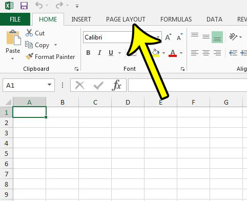
The steps in this article will show you a setting to change on your spreadsheet that will hide the lines from appearing around the cells. This refers to the gridlines. These are different than borders, which are a formatting option that can be added separately, in addition to gridlines. If you follow the steps below to hide your gridlines, but there are still lines around your cells, then you will need to remove the borders as well. This article from Microsoft can show you how to add or remove borders from Excel. Step 1: Open your spreadsheet in Excel 2013. Step 2: Click the Page Layout tab at the top of the window.
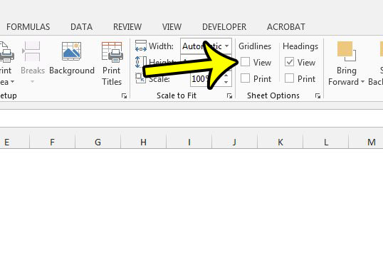
Step 3: Check the box to the left of View under Gridlines in the Sheet Options section of the ribbon to remove the check mark. The gridlines should disappear immediately. If you also would like to prevent the gridlines from appearing when you print, make sure that there is not a check mark in the box to the left of Print under Gridlines either.
Are you looking for ways to change the appearance of the printed versions of your spreadsheet? Our Excel print guide offers a number of different options and settings that you can adjust to make your document print a little better. He specializes in writing content about iPhones, Android devices, Microsoft Office, and many other popular applications and devices. Read his full bio here.